Mann-Kendall
A look into Mann-Kenall test for monotonic trend.
By Josh Erickson in R Hydrology Statistics
August 28, 2021
Intro
A lot of times in hydrology you’ll want to know whether a set of observations over time has a trend. This is usually obvious when the trend is substantial (eye-catching 👀) but less so when it is more subtle. To test the hypothesis that there is a trend we need to find a test statistic of some sort. There are a couple ways of doing this: regression coefficient or Mann-Kendall tests. Linear regression is a way of testing and is just fine (if assumptions are met) but today we’ll look into the Mann-Kendall test. The Mann-Kendall test is a non-parametric test that tests for a monotonic trend in a time series (or really any rank/ordered set). This means it is distribution free, which is very helpful if your data does not meet the assumptions of the linear regression test; however, it does need to be independent, e.g. no serial correlation. With this we’ll dive into Mann-Kendall!
EDA
I think it’s always good to bring in some data and start looking at a graph. Let’s take the annual water year peak flows from a gauging station and see what the observations look like. In the graph below it really looks like the trend is decreasing but it’s very close! This is where the Mann-Kendall (MK) test can help us make a decision; trend or no trend?
library(wildlandhydRo)
library(tidyverse)
yaak_peaks <- wyUSGS(sites = '12304500') %>% filter(!is.na(Peak))

yaak_peaks %>% ggplot(aes(peak_dt, Peak)) +
  geom_line(size = 1) +
  geom_smooth(method = 'lm')+
  labs(x = 'Peak Date', y = 'Peak Flow (CFS)', title = 'Peak Flows for USGS Station 12304500; Yaak River, MT')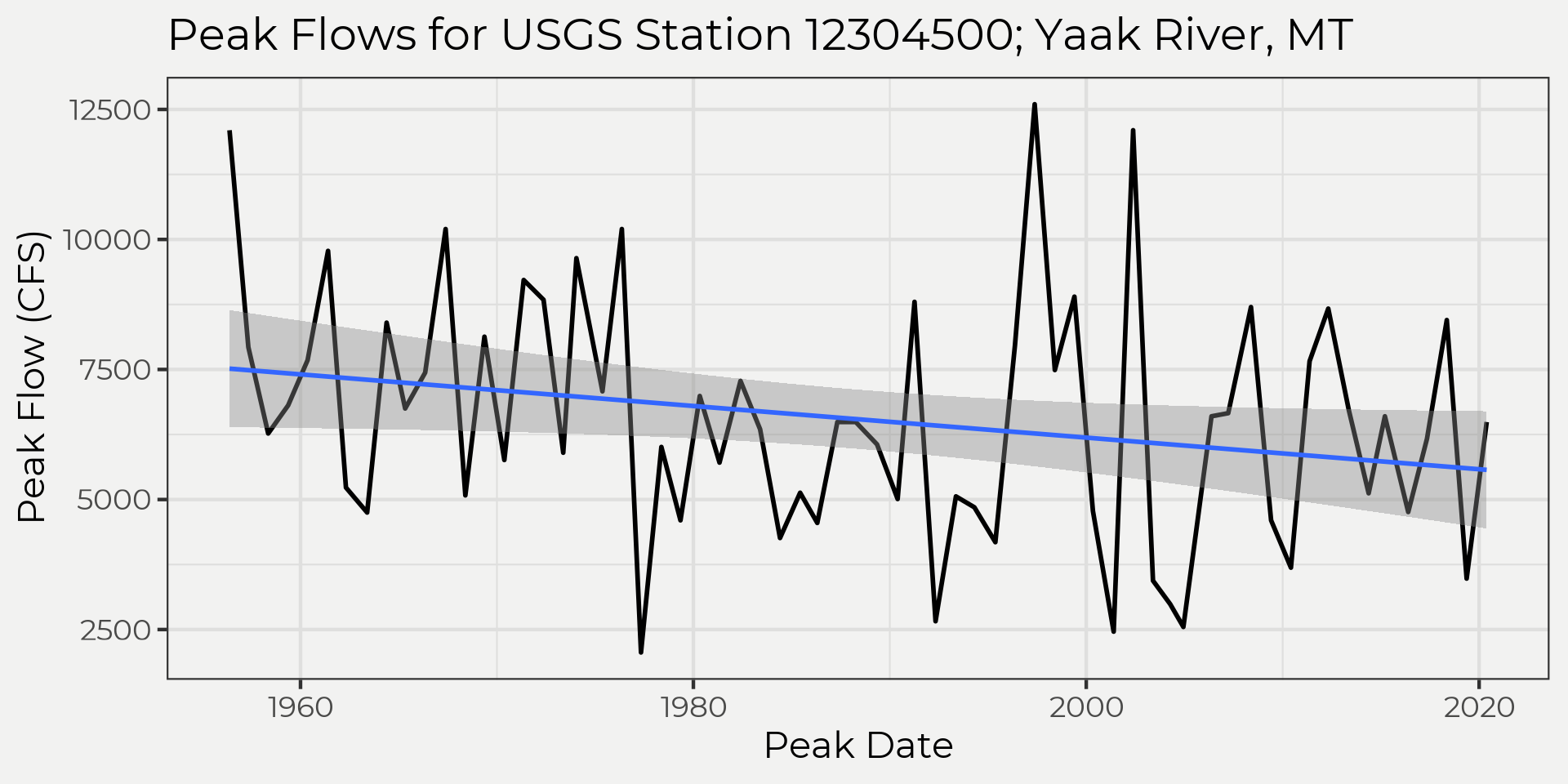
Calculating
The MK test is built around a standard normal distribution test. This is ultimately what we will be testing for, e.g. \(u_c\). Where,\[ u_c=\frac{S-sign(S)}{\sqrt{Var(S)}} \]
If \(\left|{u_c}\right|\gt Z_{(\alpha/2)}\) and \(Z_{(\alpha/2)}\) is the standard normal variate, then the null hypothesis for a trend can be rejected. We can do this because Mann (1945) and Kendall (1975) showed that \(S\) follows a standard normal distribution as well as solved for the \(\sqrt{Var(S)}\). So, how the heck do we solve for \(S\)? What is \(S\)? This is where we’ll need to dig in a little bit and understand what something called ‘\(sign\)’ does and also how to solve for \(\sqrt{Var(S)}\).
S and sign
When I first started this deep dive into Mann-Kendall I got a little hung up on the sign function aka signum. It’s a little abstract at first (IMO) but is really just a counting algorithm. At it’s core, it really is just figuring out whether a value is \(\lt 0\), \(\gt 0\) or \(= 0\). The sign function is within the \(S\) statistic. The \(S\) statistic is approximately normally distributed (remember above and solving for \(u_c\)) with a mean of 0 and a variance of \(\sqrt{Var(S)}\). Below is the equation for \(S\),
For example, let’s say we had some observations over time (important because they are ordered) and we wanted to know whether the point after (\(X(t')\)) is bigger or smaller than (\(X(t)\)) we could just take \(X(t')-X(t)\) and if it’s negative it means it’s smaller and if it’s positive it means it’s bigger (also 0 if they’re equal). But let’s say we do this as a rolling subtraction, e.g. \(x_1-x_1, x_2-(x_1, x_2),x_3-(x_1, x_2,x_3),\dots, x_n-(x_1,\dots,x_n)\). Now if we did this for each point as we progress to the end we would have a lot of positive and negative values and maybe some equal results right? In the code below you can see that this is what is going on, that is we are subtracting but rolling in time from the beginning to end.
x <- yaak_peaks$Peak
n <- length(x)
S <- 0.0
for(j in 1:n) {
    S2 <- list(data.frame(rolling_sub = x[j] - x[1:j], name = paste0(j)))
    S <- append(S, S2)
  }
head(S)
## [[1]]
## [1] 0
##
## [[2]]
## rolling_sub name
## 1 0 1
##
## [[3]]
## rolling_sub name
## 1 -4170 2
## 2 0 2
##
## [[4]]
## rolling_sub name
## 1 -5830 3
## 2 -1660 3
## 3 0 3
##
## [[5]]
## rolling_sub name
## 1 -5290 4
## 2 -1120 4
## 3 540 4
## 4 0 4
##
## [[6]]
## rolling_sub name
## 1 -4420 5
## 2 -250 5
## 3 1410 5
## 4 870 5
## 5 0 5Let’s take a closer look in the graph below. The data.frame below S is just taking the peaks and subtracting \(X(t')-X(t)\) in this rolling pattern which inevitably is getting larger and larger samples as time goes on, e.g. \(x_n-(x_1,\dots,x_n)\). As you can see, values with more blue tend to be higher than values with more black. This will matter in the next steps.
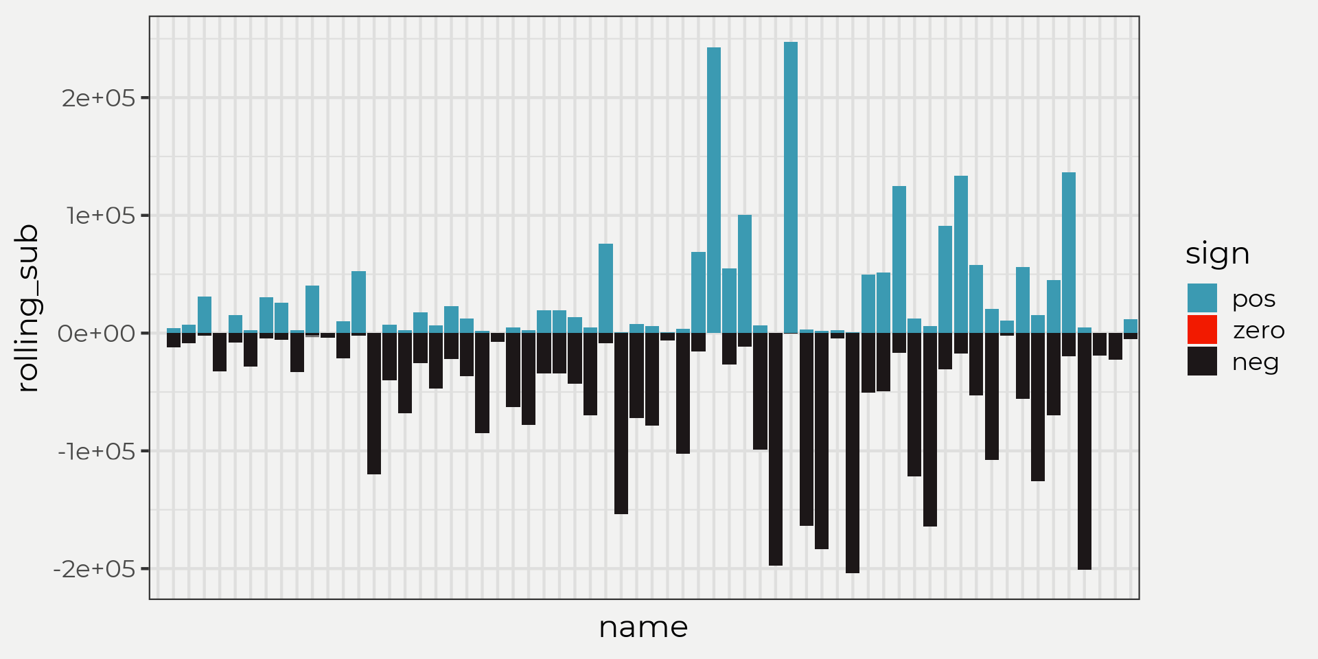
Ok, the next step would be to add them up right? Well, sure but sign does this in an pretty cool and effective way that doesn’t let outliers drive the final results. Remember, the sign function is a counting method and all it does is determine whether the value is -, + or 0 and then gives either a -1, 1 or 0 as a result! By doing this the sign() makes it easy to interpret all of the -, + and 0’s.
\[ sign(a)=\begin{cases}\frac{a}{\left|a\right|}, & \text{if} \ x \neq 0 \\ 0, & \text{if} \ x = 0 \end{cases}=\large\begin{cases}1, & \text{if} \ a \gt 0 \\ 0, & \text{if} \ a = 0 \\ -1, & \text{if} \ a \lt 0 \end{cases} \]
So if we do this to the graph above we can see what each iteration expresses in terms of lower, higher or equal to in point graph. The point graph is a intuitive graphic for me in this problem because S is essentially a reflection of ‘the more +, - or 0’s you have as time goes on, the more this will determine your trend’.
sign_it <- S_df %>%
  group_by(name) %>%
  nest() %>%
  mutate(sign_result = map(data, ~sign(.$rolling_sub))) %>%
  select(name, sign_result) %>%
  unnest(sign_result) %>%
  ungroup()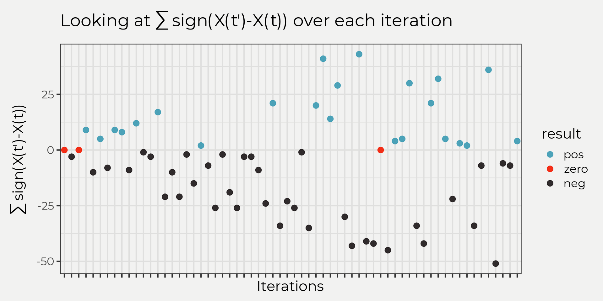
So the next step in solving for \(S\) is to sum up all of those points! This will give us a final sum and an reflection of a trend, e.g. more negative means downward and more positive means upward and closer to zero means no trend!
sum(sign_it$sign_result)## [1] -373Now if we look at the Kendall::MannKendall() function you’ll see we get the same answer. How cool is that!?
#Mann-Kendall function S score

Kendall::MannKendall(yaak_peaks$Peak)$S[1]
## [1] -373\(\sqrt{Var(S)}\)
Now let’s move on to the variance part of the \(S\) equation. The \(VAR(S)\) will help us finish the \(S\) and also give us an idea of the what’s going on with the variation in the data. To solve for \(VAR(S)\) we need to use the equation below,
\[ VAR(S)=\frac{1}{18}\left[n(n-1)(2n+5)-\sum_{p-1}^{g}t_{p}(t_{p}-1)(2t_{p}+5)\right] \]
where \(n\) is equal to the sample size and \(t_p\) is equal to repeated values in the sample. Most of the time in hydrology we will not get repeated values when we sample but in this example we did so we’ll need to account for those repeats using \(\sum_{p-1}^{g}t_{p}(t_{p}-1)(2t_{p}+5)\) above, e.g. peaks that are the same. There are also some rules for sample size where \(n \le 10\) will need to use a table of probabilities and not perform \(VAR(S)\) but most of the time you’ll have over 10 samples (i hope 😉).
yaak_peaks %>% count(Peak) %>% filter(n>1)## # A tibble: 5 x 2
## Peak n
## <dbl> <int>
## 1 4600 2
## 2 6490 3
## 3 6600 2
## 4 10200 2
## 5 12100 2FYI you won’t use \(\sum_{p-1}^{g}t_{p}(t_{p}-1)(2t_{p}+5)\) if there are no repeats in the time series and will just solve for \(\frac{n(n-1)(2n+5)}{18}\).
So let’s solve for \(VAR(S)\)! We’ll need the length of the vector to get \(n\) and we’ll need to perform the summation of the repeated values.
n <- length(yaak_peaks$Peak)
repeats <- yaak_peaks %>% count(Peak) %>% filter(n>1)

repeat_res <- vector()
for(i in 1:length(repeats$n)){
  rr <- repeats$n[i]*(repeats$n[i]-1)*(2*repeats$n[i] + 5)
  repeat_res <- append(repeat_res, rr)
}

var_s <- (1/18)*(n*(n-1)*(2*n+5) - sum(repeat_res))
var_s
## [1] 31192.33And now if we look at the Kendall::MannKendall() result we can see that they are the same!
Kendall::MannKendall(yaak_peaks$Peak)$varS[1]## [1] 31192.33With that we can now complete the equation for \(S\)!
Findings
So we went through the details of solving for \(S\) and now we need to bring it all back together. Remember,
\[ u_c=\frac{S-sign(S)}{\sqrt{Var(S)}} \]
That means we can now plug in the numbers from above and find out what \(u_c\) is!
u_c <- (sum(sign_it$sign_result)-sign(sum(sign_it$sign_result)))/(sqrt(var_s))From here, since \(u_c\) follows a normal distribution we can test whether \(\left|{u_c}\right|\gt Z_{(\alpha/2)}\). To do that we’ll just use the code below.
z_alpha_div_2 <- qnorm(0.95, mean = 0, sd = 1)

abs(u_c) > z_alpha_div_2
## [1] TRUEp_value <- 2*pnorm(-abs(u_c), mean = 0, sd = 1)
p_value## [1] 0.03517881Thus, we can reject the null hypothesis at a significance level of 0.05 that a trend exists.
The easy way
Most of the time (all) you will just run a Mann-Kendall type function and get the results of your test via a p value. Like in the code below, the print out says that we have a p value of 0.0352 and if we set our \(Z_{\alpha/2}\) to 0.05 then we can reject the null!
Kendall::MannKendall(yaak_peaks$Peak)## tau = -0.18, 2-sided pvalue =0.035179As you can see it is the same as the example above with p_value. Now we can say that the peak flow are trending down!

Conclusion
When using Mann-Kendall test to find a trend in a time series just remember that the data shouldn’t be autocorrelated (serial correlation) and it’s good to have at least more than 10 samples. From there, it’s a counting method (signum) that figures out how much the observations move +, - or don’t change over time. Since it’s normally distributed (\(S\)), we can test whether the value \(S\) is statistically significant or not using the standard normal distribution! Hope this helps! Until next time.
References
Kendall, M. G. (1975). Rank correlation methods. 2nd impression. Charles Griffin and Company Ltd. London and High Wycombe.
Mann, H. B. (1945). Nonparametric tests against trend. Econometrica: Journal of the econometric society, 245-259.