Hydrology Distributions: Part II

Goals

• see some different pdf equations
• explore visually
• check assumptions
• frequency of occurrence

Theoretical PDF’s

I know it’s a lot but I think it’s helpful to just see the different pdf’s (\(f_{x}(x)\)) written out symbolically. If we remember from part I (normal distribution) there are parameters that we need to sample from our data and then we can enter them into the pdf. That is essentially the beautiful mess below (parameters for different pdfs). Thus, we’ll look at the following distributions below: normal (N), Lognormal (LN), Log-Pearson Type III (LP3), Pearson Type III (P), Gumbel (G), Weibull (W) and Generalized Extreme-value Distribution (GEV).

So what do these things look like with real data? That is to say, what would these pdf’s produce if we fed it some observations? Well, that is what we’ll look into in the next part! Visualizing! These equations above are just pdf’s. That’s it! If you have observations you can then feed these observations into the equations above. We’ll start to see below how some look better than others though.

Visualizing

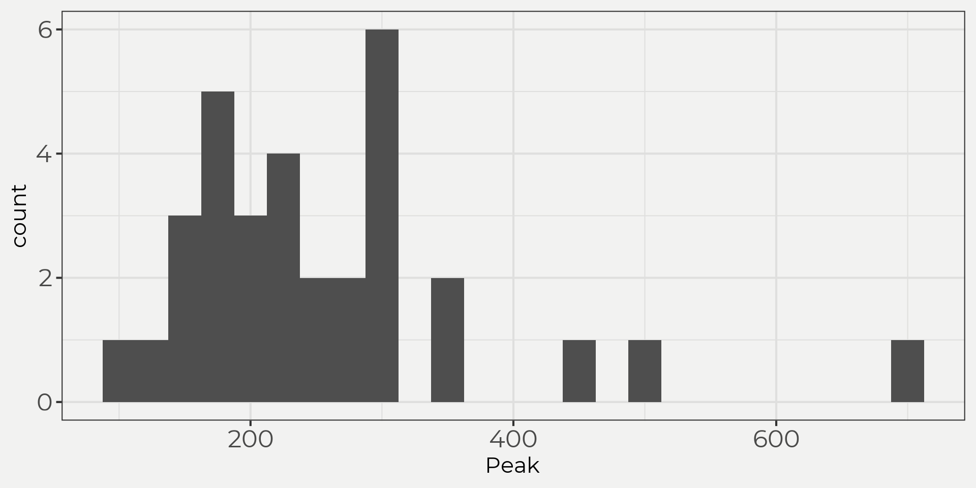
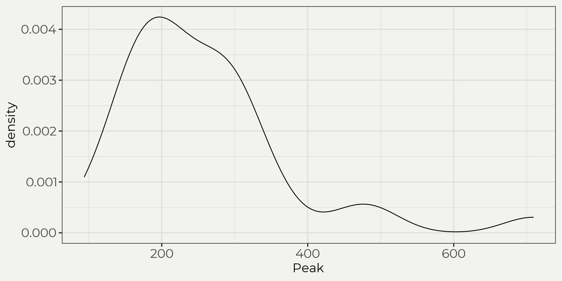
To do this let’s bring in a set of peak flows from a USGS gauging station. Then we can start to view the data in a few different ways: time series, histogram and density plots.

flower_peak <- wildlandhydRo::wyUSGS(sites = '12303100')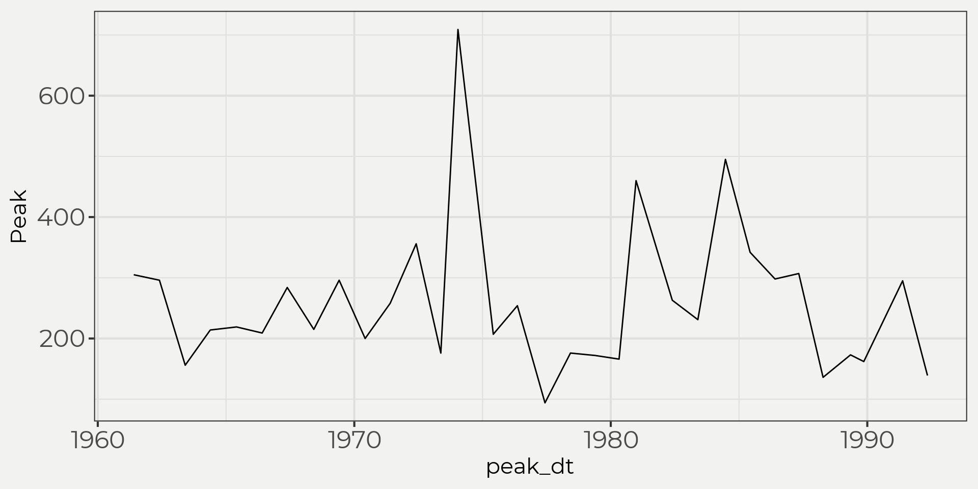

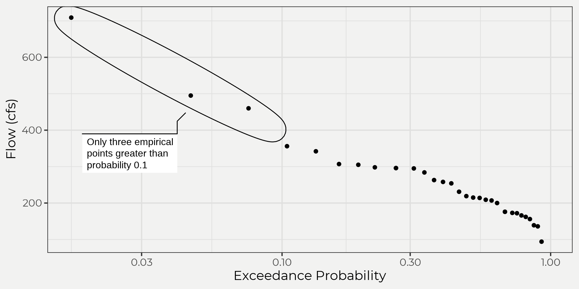
Visualizing Plots of Peak Discharge in Different Ways

So what would happen if we just took the probabilities of the empirical data? Like, why do we need to fit a distribution anyways? Good point! We can find probabilities with our data and should! However, most of the time you’ll want to fit to a distribution because you want to estimate a rare event and you don’t have enough data collected. So, let’s check out our data. We’ll use the code taken from JP Gannons’ book/lectures and use the Gringorten plotting position formula. For more information on exceedance probabilities check out the JP Gannons’ site or for other plotting position methods. Side-bar, just like anything in statistics this can get deep fast and very pedantic! So please be aware that this is just a quick look and there are plenty of reasons you might want to change plotting position methods, e.g. distribution, a priori, length of record, pedantic, etc.

Gringorten plotting position

\[ q_i = \frac{i-a}{N+1-2a} \\ \displaystyle{\text{where,} \\ q_i = \text{Exceedance probability}\\ N = \text{Number of observations in your record}\\ i = \text{Rank of specific observation, i = 1 is the largest, i = N is the smallest.}\\ a = \text{constant for estimation = 0.44} }\]

We’ll just apply this to our data and get an idea of what the probabilities are.

exceed_flower <- wildlandhydRo:::get_exceedence(flower_peak$Peak)

Below we can see the results of our stations exceedance probabilities and associated flows. Notice how it only goes to 0.0164127 probability which is equivalent to a 61 year return interval! This is not good if we wanted to know the 0.1 probability of exceeding a associated flow aka 100 year event. We would need to fit a line and then extrapolate beyond our domain. Wait, what?! Yeah, I know we shouldn’t do that! But, we can get around that by substituting with a theoretical distribution 😉.

Now that we know we need to fit to a theoretical distribution (since we want to go beyond) we can start to explore the pdf’s from above. The goal is to see if we can find something close. To do that we’ll need to fit our empirical data (flower_peak) to a theoretical one. Plug and chug, right? Well, what the heck. Yes! The only reason I say that is it gets a little nutty when you dive into sample statistics and parameter estimation IMO. So for this example we’re going to spare ourselves on the math side and just have the computer do the fitting for us.

We can do this pretty fast with the help of a few packages: {fitdistplusr}, {extRemes}, {smwrBase}. I wrapped these up in a function called batch_distribution() in the {wildlandhydRo} package. The function will fit our data to different distributions and then we can plot them against each other. Some will be off and some close.

library(smwrBase)
library(evd)

flower_dist <- flower_peak %>% wildlandhydRo::batch_distribution(Peak)

wildlandhydRo::plot_densDist(flower_dist, facet = F) + geom_density(data = flower_peak, aes(Peak, linetype = 'Empirical'), size = 2, key_glyph = 'path',bw = 50) + scale_linetype_manual(values = c('Empirical' = 2), label = '') + labs(linetype = 'Empirical') + theme(axis.text = element_text(size = 18))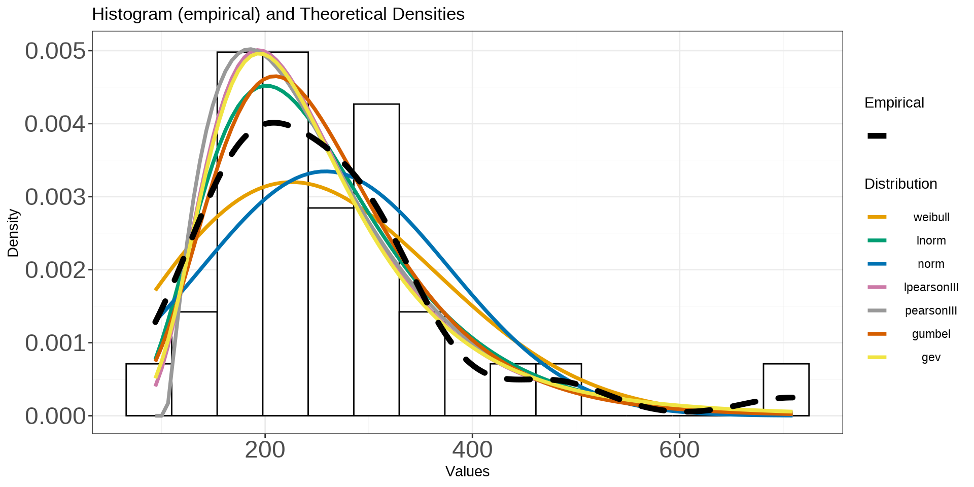

The graph above shows us both the empirical against the theoretical distributions. What’s nice about this is we can start to see what it means by ‘fit a distribution’ to the empirical. This is an important step in frequency analysis as it will determine what you use for your final probabilities/results. As we can see, there are a couple distributions that are a little different than the others (weibull and normal) and a few that look really close (GEV, log Pearson and Pearson) to the empirical distribution.

The idea is that the more data we collect the more a theoretical distribution will fit to our empirical data. We can see that some distributions are underfitting and overfitting! We can also see this in a Q-Q plot like below.

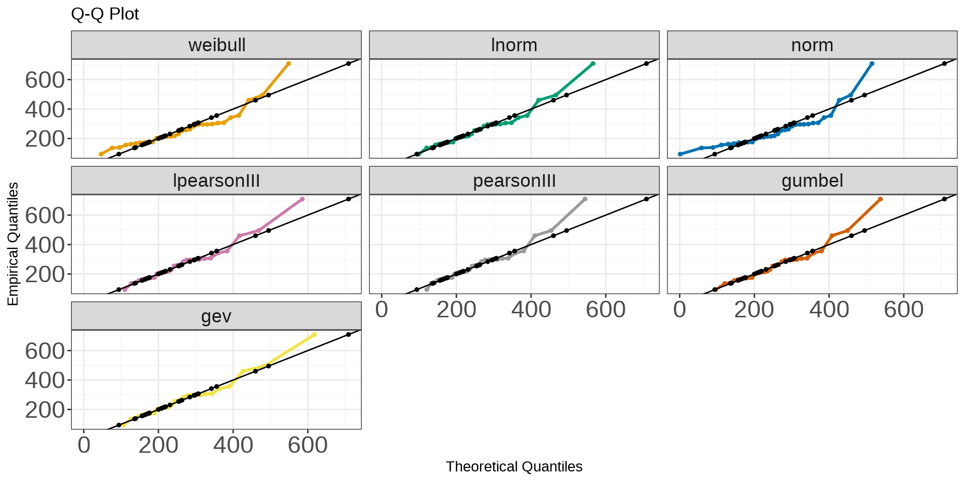
You can see that some distributions again are a little better at representing the empirical data but all of them underestimate the right-tail of the data. What distribution should we use then? This is where we need help and would need to use some hypothesis testing for ‘goodness of fit’ (GOF), domain expertise and a little more exploration into parameter estimation but we’ll deal with that in part III. Just remember though that these are just pdf’s (part I) and we use our sample data to estimate plug-in. That’s it!

Assumptions

One key component of using theoretical distributions is the underlying data follows some assumptions; iid and stationarity. We’ll do a quick test for stationarity and then talk through iid. Below we’ll test for stationarity using the Dickey-Fuller test (Fuller, 1996). What we are trying to find is whether the mean and variance change over time. If they don’t then the data is assumed stationary. Most annual maximum series (AMS) in hydrology follow the stationarity assumption; however, with recent climate change or other factors (jump, land management) these assumptions cannot be assumed so it’s always good to check (Maity, 2018).

library(tseries)

flower_stationarity <- flower_peak %>% 
  filter(!is.na(Peak))

adf.test(flower_stationarity$Peak, k = 1)

## 
##  Augmented Dickey-Fuller Test
## 
## data:  flower_stationarity$Peak
## Dickey-Fuller = -3.1453, Lag order = 1, p-value = 0.131
## alternative hypothesis: stationary

Since the hypothesis test was above the threshold we set (I promise we set it at 0.05 😆) then we can’t reject the null. Now we need to make sure our data is iid. We are doing AMS so autocorrelation is not a problem so we can assume our data is independent. However, for the identically distributed assumption we need to make sure our peak flows are from the same distribution. That is to say, the flow regime needs to be the same. We can explore this by looking at the different times these peak flows happened, e.g. winter rain-on-snow (ROS), spring snowmelt, summer-fall rainstorms.

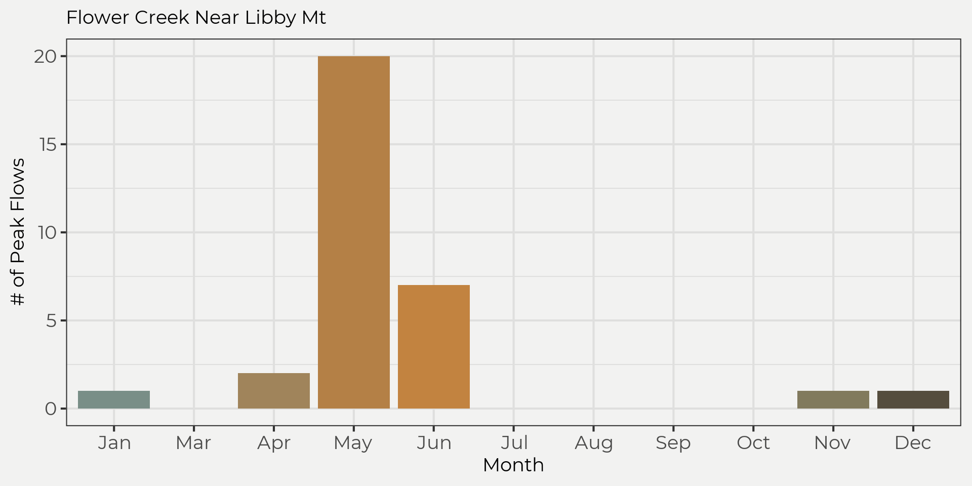
We can see that most of the peak flows are in the snowmelt regime but there are a few that are from the ROS. Since these are from two different populations we need to take one out to proceed with the frequency analysis. Now if we take the ROS out and only look at the snowmelt regime then we can meet our assumptions.

flower_peak_snow <- flower_peak %>% 
  mutate(month = month(peak_dt)) %>% 
  filter(!is.na(Peak), 
         month %in% c(4,5,6))

adf.test(flower_peak_snow$Peak, k = 1)

## 
##  Augmented Dickey-Fuller Test
## 
## data:  flower_peak_snow$Peak
## Dickey-Fuller = -2.8654, Lag order = 1, p-value = 0.2408
## alternative hypothesis: stationary

We now have some new competitors…

flower_dist_snow <- wildlandhydRo::batch_distribution(flower_peak_snow, Peak)
wildlandhydRo::plot_qqDist(flower_dist_snow, facet = T) + geom_point(data = flower_peak_snow, aes(Peak, Peak), size = 1) + theme(axis.text = element_text(size = 18),
                                                                                                                       strip.text = element_text(size = 14))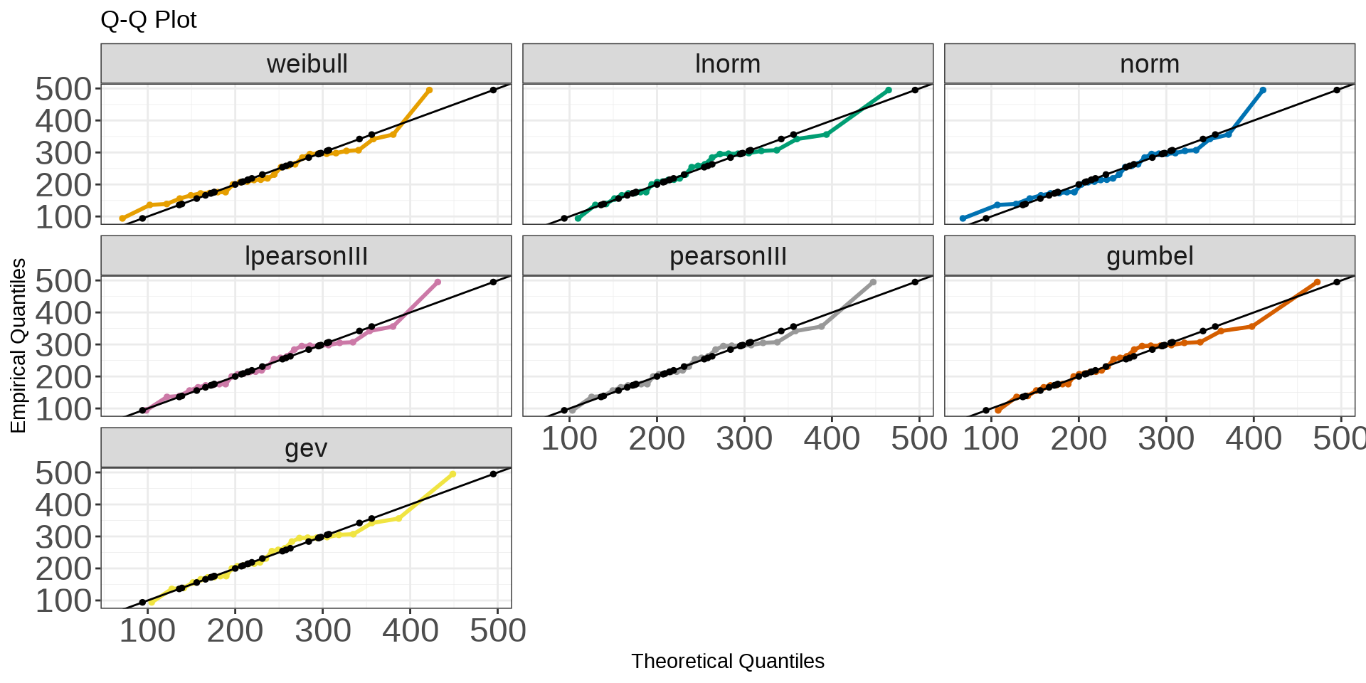

Looks like the Gumbel distribution is possibly the best fit (eyeballing) so let’s use that in the following examples.

Frequency of Occurrence

So why do we even care about pdf’s in hydrology? Well, a lot of times we will use these pdf’s to calculate frequency of occurrence aka probability of occurrence aka annual return interval (ARI) aka annual exceedance probability (AEP). What the heck! Yeah I know, there are a lot of ways people say the same thing 😉. These probabilities give us a statistical understanding of discharge and it’s probability of occurring during a water year. From that, we can use for planning, risk and reliability of hydrologic design. There are a few different ways to calculate probability of occurrence (univariate pdf’s): plotting position (mentioned earlier), plug-into pdf (part I) or frequency analysis and probably others 🤷. Frequency analysis is pretty intuitive and it will look really familiar to something in part I (Z-score) but is referred to as the general equation of frequency analysis (Maity, 2018). Essentially we are going to calculate for the value (flow in our case or \(X_T\)) given by

general equation of frequency analysis

\[ X_T = \overline{X} + KS \\ \displaystyle{\text{where,} \\ X_T = \text{magnitude of the hydrologic variable with a return period of}\ T; \\ \overline{X} = \text{mean of the hydrologic variable}; \\ S = \text{standard deviation of the hydrologic variable; and} \\ K = \text{frequency factor, a function of the return period} \ T\ \text{and the assumed frequency distribution function}} \]

This looks really similar to the classic Z score for a normal distribution, right?

Z score

\[ Z=\frac{(\text{value} - \overline{x})}{s^2} \leftrightarrow Zs^2 + \overline{x} = \text{value} \]

\[ \displaystyle{\text{where,} \\ Z = \text{frequency factor (aka K)} \\ \text{value}= \text{magnitude of the variable aka} \ X_T} \]

That’s because it is! We are just now solving for a value (\(X_T\) magnitude with reoccurrence interval) instead of the \(Z\) or \(K\) value. Below we’ll work through an example using a Gumbel distribution. Step-by-step.

Solving

To solve for \(X_T\) we are going to need a few things; \(\overline{X}, Z, K\). Let’s start with the \(\overline{X}\). This is just the mean of the series!

mean_flower <- flower_peak_snow %>% 
  pull(Peak) %>% mean()

Now that we got \(\overline{X}\) let’s solve for \(K\). This is just the standard deviation of the series.

sd_flower <- flower_peak_snow %>% 
  pull(Peak) %>% sd()

For the final variable \(K\), we’ll need to find the frequency factor for the Gumbel distribution. Below we’ll use the formula from Al-Mashidani & Mujda (1978) to find \(K\) by using 0.1 probability or \(T=10\) as our point estimate.

Formula for Gumbel K

\[ K=-\Bigg[\frac{(6)^{\frac{1}{2}}(0.5772 + \text{lnln}\ T/T -1)}{\pi}\Bigg] \]

#find K
k_flower <- -(((6^.5)*(0.5772 + log(log(10/(10-1)))))/pi)

So we’ll want to compare the plotting method with the frequency analysis to see if our graphs were right and we’re not way off the mark. As you can see below, they are really close. This is good 👍!

#solve for frequency analysis
frequency_analysis <- mean_flower + k_flower*sd_flower

frequency_analysis

## [1] 346.7417

#now show exceedance probability
exceed_flower %>% filter(exceedance_probability <= 0.11,
                         exceedance_probability >= 0.09) %>% 
  pull(x)

## [1] 356

Or the easy way is to use the evd::qgumbel() function to find the flow at that recurrence interval, see below. We’ll use the batch_distribution() object from earlier, e.g. flower_dist_snow().

loc_flower <- flower_dist_snow$gumbel$estimate[['loc']]
scale_flower <- flower_dist_snow$gumbel$estimate[['scale']]

flower_at_10yr_ari <- evd::qgumbel(0.9, loc = loc_flower, scale = scale_flower)
flower_at_10yr_ari

## [1] 352.0953

Now let’s do what we set out to do and extrapolate! Remember we wanted to see what a 100-year return interval (aka ARI) would give us and now we can do that. We’ll use the theoretical distribution to get us there. We just enter the equivalent to a 100 ARI (e.g. \(ARI = 1-\frac{1}{T}\)) in the {evd} equation above and we get back the estimated flow!

flower_at_100yr_ari <- evd::qgumbel(0.99, loc = loc_flower, scale = scale_flower)
flower_at_100yr_ari

## [1] 509.2854

Pretty cool. We can take it a step further with the wildlandhydRo::batch_frequency(). This will give us some probabilities up to 0.005 but of course you can always go further if needed.

flower_ff <- wildlandhydRo::batch_frequency(flower_peak_snow, Peak)

flower_ff %>% 
  filter(Distribution == 'Gumbel') %>% 
  ggplot(aes(ReturnInterval, Value, color = Distribution)) + 
  geom_point() +
  geom_line() +
  labs(x = 'Return Interval', y = 'Discharge (cfs)', title = 'Return Intervals using a Gumbel Distribution')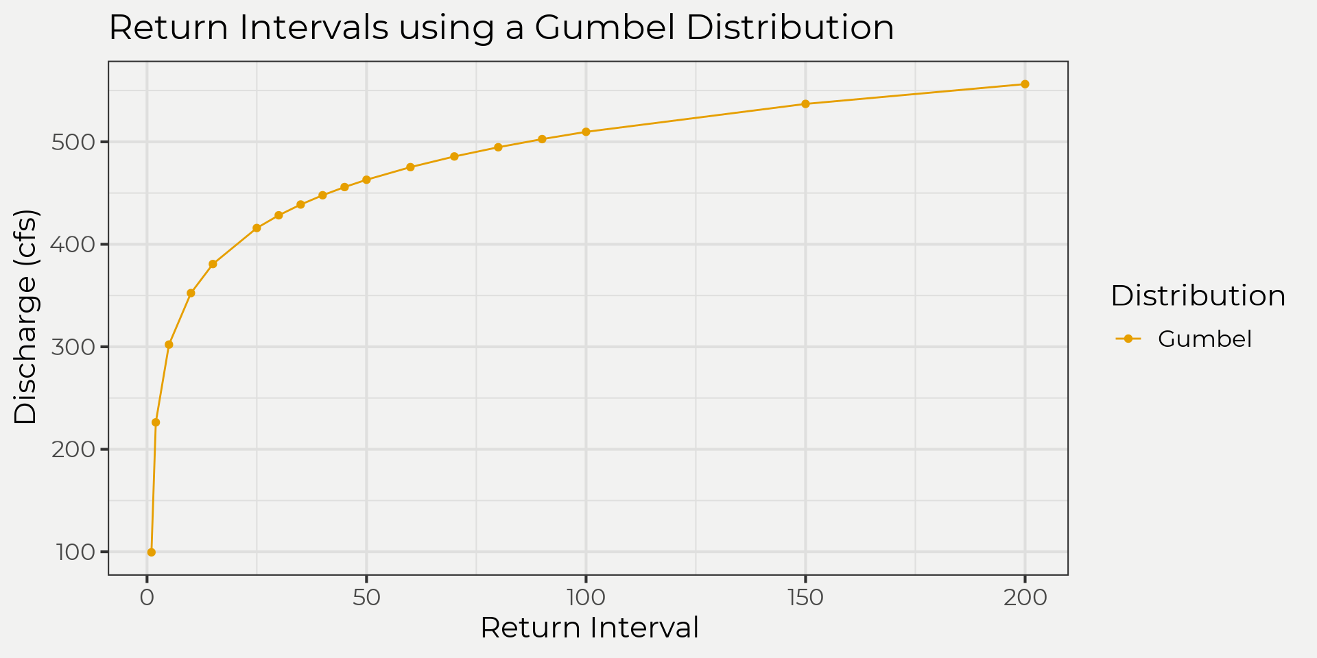

Wrap it up

So we were able to take some hydrological data (stream flow annual peaks/maximums) and see how this data looks with different theoretical distributions. From there we explored different ways of getting probabilities and why we might want to use a theoretical distribution. Wrapping up we looked at a few ways to get that information. I hope that this was a nice overview of some hydrology distribution stuff! If you have any questions or comments give me a shout. In the next blog post we’ll look at the ‘what’ dististribution should we use.

References

Al-Mashidani, G., LAL, P. B., & MUJDA, M. F. (1978). A simple version of Gumbel’s method for flood estimation/Version simplifiée de la méthode de Gumbel pour l’estimation des crues. Hydrological Sciences Journal, 23(3), 373-380.
Maity, R. (2018). Statistical methods in hydrology and hydroclimatology. Springer.
Fuller, W. A. (1996). Introduction to Statistical Time Series, second ed., New York: John Wiley and Sons.